How to accurately predict NBA player stats

Our technical series continues with three methods for projecting a player's stats

Player stats are fairly volatile — more volatile than fans realize — as they depend on many external factors and lots of random chance.

Some statistics stabilize quickly, such as 2-point percentage and rebounding rate. Others, like 3-point percentage, can take years to settle.

Naturally, when creating advanced NBA metrics, we want to determine a player’s true skill level. Estimating this accurately is the key to building metrics from box-score statistics, similar to Box Plus-Minus (BPM) and some other all-in-one stats.

Today, I’ll cover three methods based on statistical and machine-learning techniques for estimating a player’s true skill level for virtually any individual statistical category.

We can use these methods for percentage-based stats — 3-point percentage is an example — or for per-possession stats, such as assist rate.

Additionally, these methods allow us to create confidence intervals — essentially a range in which we’re relatively certain the player’s skill resides.

---

---

An example

Imagine a rookie coming into the NBA and making 5 of his first 10 attempts from 3-point range. Obviously, if we are projecting his performance forward, it’d be unwise to expect him to continue to make 50% of his 3s.

But what’s our best guess? And how narrow can we make our prediction of his true skill?

When it comes to 3-pointers, previous analysis has found out that 750 3-point attempts are necessary before signal outweighs noise (random chance).

But that is far from saying the first 750 3s provide no information: We can say more about a player who shot 10-for-20 than about someone who shot 5-for-10.

---

For Part 1 of our series on creating advanced stats, click here:

---

Prior information

Even before a new player enters the league, we have enough data to predict the likely range of his stats — for example, we know that NBA players hit about 36% of their 3-pointers overall, while virtually no players hit more than 50% consistently.

Plotting the distribution of NBA player 3-point shooting in a histogram, we get the following picture, showing a realistic range of 22% to 45%.

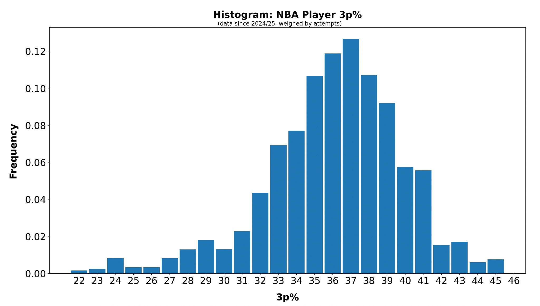
For any player, it makes sense to assume that his skill lies somewhere within the above distribution, with the extremes on the left and right being less likely: It’s more likely for an NBA player to be a 36% shooter than a 31% or 41% one.

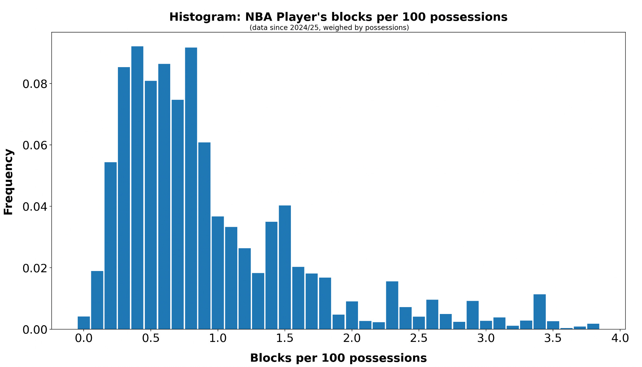
Depending on the statistic in question, the player distribution can vary greatly. Here is a histogram for blocks per 100 possessions:

---

Three different approaches

1. Penalized regression and machine learning

Most machine learning algorithms — from regression to neural networks — require us to transform the data into an X matrix and a “results vector” called y.

In our 3-point shooting example:

y: Holds the outcomes of each shot (makes and misses), coded as ones and zeros.

X: Holds the variables. As with Adjusted Plus-Minus (APM), we use “dummy variables” to denote a player’s presence on the court, also represented by ones and zeros.

The number of columns in the X matrix equals the number of players in the dataset, with each column corresponding to one specific player. Each individual 3-point shot — whether a make or a miss — is an “observation” and gets its own row.

For a player who goes 5-for-10, the X-matrix and results vector would look like this:

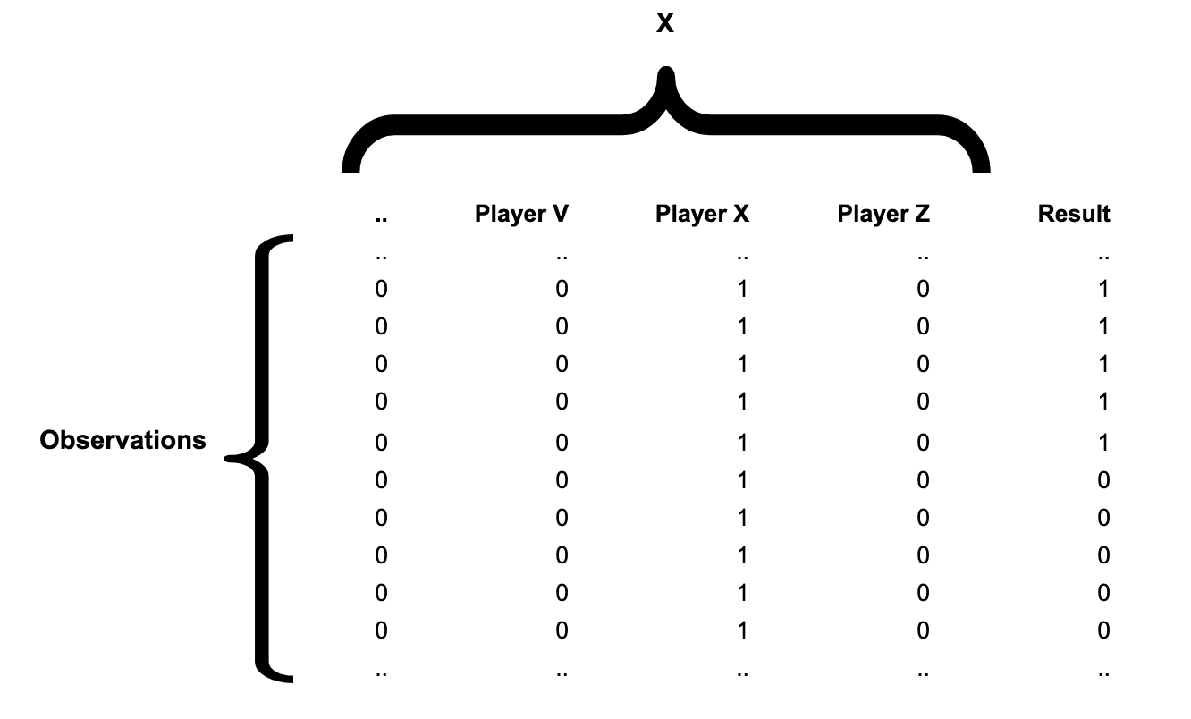
Since the X-matrix is even sparser than the one used in APM — it contains only a single “1” per row — it makes sense to use sparse matrices if your programming language supports them.

If we used a standard least-squares regression, the coefficient for our example player would be 0.5. With no constraint put on the coefficient, it ends up fitting the data perfectly. But we know the 50% figure is not a good prediction of that player’s true skill.

To get more accurate predictions, the methods below use penalization. Through internal cross-validation, they determine how strongly to pull coefficients toward the league average, and whether they should penalize strong deviations linearly, quadratically, or a mix between the two.¹

clf_el = linear_model.ElasticNetCV()
clf_lasso = linear_model.LassoCV()
clf_ridge = linear_model.RidgeCV(alphas = [..])
clf.fit (X, y)

Note that, for many of the ML algorithms to perform better, we need to put everyone’s attempts into X and y, even if we’re interested in the skill of just one player. This will allow the algorithms to more accurately determine the optimal penalization.

Using the above Ridge Regression setup, we get the following estimates for some select players:

Employing the technique laid out by Justin Jacobs allows us to also compute the 95% confidence intervals.

Plotting attempts against the uncertainty of each player’s skill estimate, we see how a larger number of attempts leads to less uncertainty but that the downslope flattens out with more attempts.

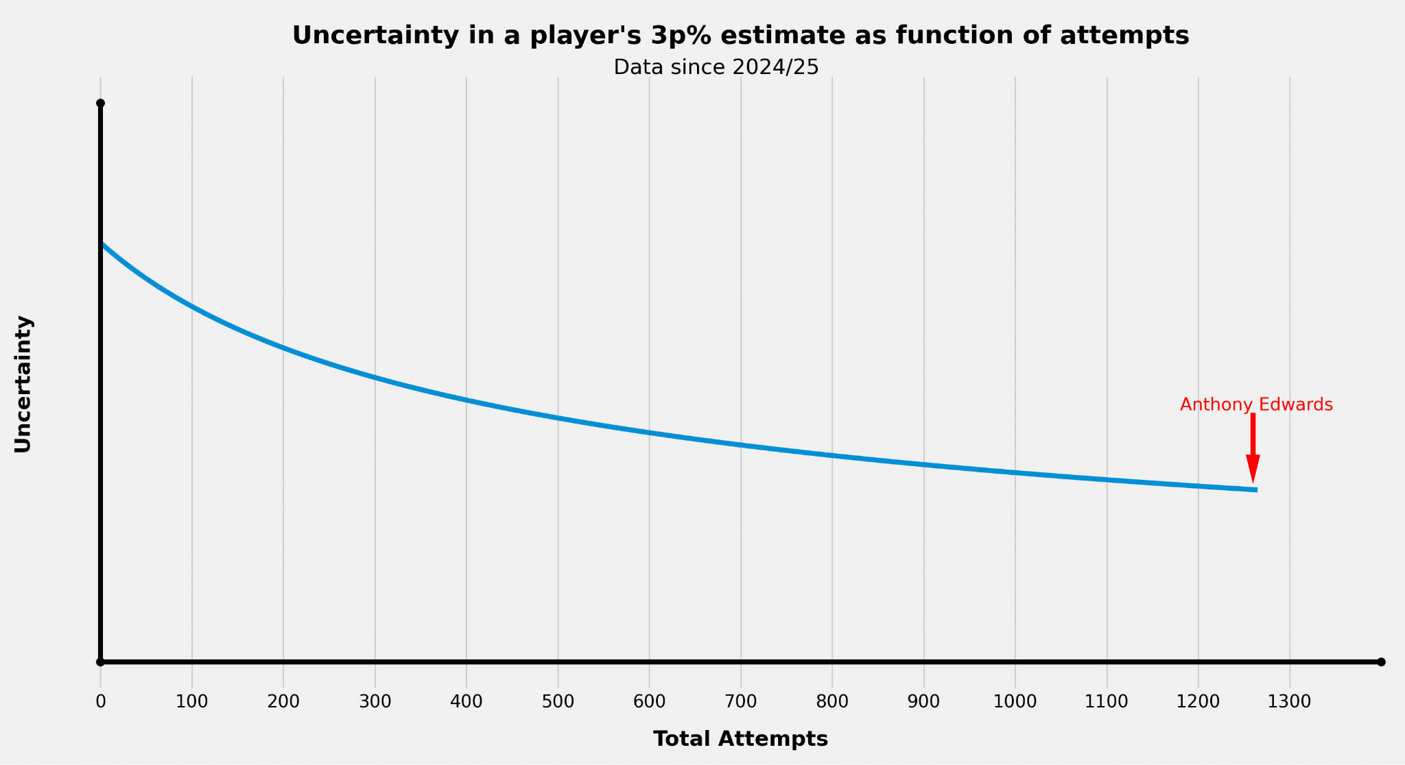
Initial attempts help us narrow down the player’s true ability more than attempts when we already have a decent sample.

---

Optimizing with weights

To save memory and processing power, we can take advantage of the fact that many rows in our matrix are identical. Instead of repeating them, we can weight the rows by the number of occurrences.

Python’s sklearn’s Ridge function allows for weighing observations like this:

clf.fit(X, y, sample_weights = [.., 5, 5, ..])

Or we can weigh them “manually:”²

for i in range(0, numpy.shape(X)[0]):
  X[i] *= sqrt(occurances)
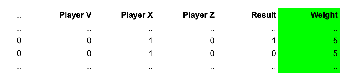
  y[i] *= sqrt(occurances)

With huge amounts of space saved — instead of thousands of rows per player, we need only two — we can now also use the method for per-possession statistics. To do so, we replace the numerator and denominator from the 3-point analysis — makes and attempts — with blocks and possessions:

As an example, let’s use a player with 20 blocks in 1,000 possessions:

The initial X-matrix stays the same, but the weights change to 20 and 980, with 20 representing the number of possessions with blocks, and 980 representing the possessions without a block.

If we do any of the above regression techniques, we then have to calculate new penalization parameters, since these are going to be different for every statistic.

---

Two ways to further improve projections

(1)

In our technical article explaining RAPM, we showed how to incorporate priors. Priors represent an initial first guess about our variables. Depending on the statistic, this can be a helpful tool.

Take, for instance, block rate. If we create two histograms — one for the taller half of the NBA, and one for the shorter half — we can easily see that the distribution appears to be dependent on height.

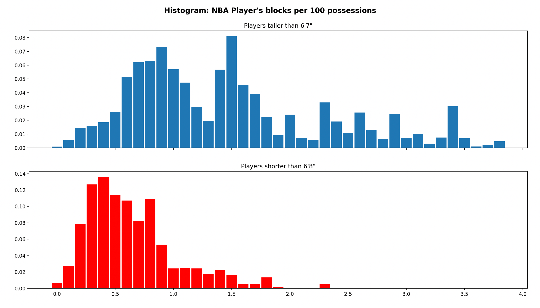
Other stats, like steals or points, might show distributions dependent on age.

So, rather to have an implied “zero” prior for everyone, it seems intuitive to create individual priors based on player attributes.

Some considerations have to be made regarding how to model these relationships, such as deciding on the size of the buckets.

(2)

A technique that aims to estimate a player’s skill level “in a vacuum” (as if he were playing for an average team) is to adjust for impact of teammates.

Most people would agree, for instance, that it’s easier to sport a good shooting percentage when playing with Nikola Jokić or Luka Dončić compared to playing on this year’s Wizards team. And playing alongside Victor Wembanyama might cost his Spurs teammates some defensive rebounds.

To adjust for this, we can introduce a second set of variables to our X-matrix.

The first set denotes the player’s own ability.

The second set of variables has the same size: the total number of players. But the dummy variables within this subset denote whether a specific teammate was on the court.

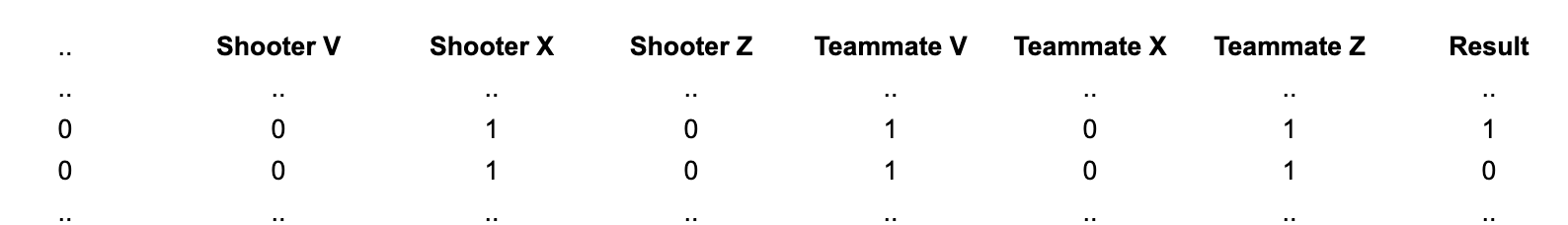
The coefficients of these new variables denote the size of each player’s teammate effect.

Using cross-validation, we can compute different penalization values for each variable type.

When we run this analysis for points per shot, we see several high-usage players at the top when it comes to positively influencing their teammates’ efficiency:

---

---

2. Using combined probabilities

For this method, we are going to use the information represented in the 3-point percentage histogram above.

We can easily compute the average and standard deviation for the above player population using traditional methods, but let’s use a probabilistic method — Monte Carlo simulation — to compute these two numbers, as the method will come in handy later:

Using a (uniform) random number generator, we draw a number on the histogram’s X-axis and create two lists:

1. Contains the 3-point percentage drawn (the number on the x-axis)

2. Contains the probability of that 3-point percentage, according to the histogram (the number on the y-axis). This second list can be viewed as weights.

We then calculate a weighted average and standard deviation. This will lead to the exact same results as usual methods, assuming we draw a sufficient number of times.

But so far, we haven’t made use of the 3-point data of the player in question. To do so, we have to modify the second list:

For every number drawn from the x-axis, we compute the probability of this number leading to the exact number of makes, given the number of attempts.

Taking our example player who went 5-for-10 on 3s:

If we first draw “37%” on the x-axis, we compute the probability of a 37% shooter going 5-for-10, and so on. The probability of drawing 37% multiplied by the probability of a 37% shooter going 5-for-10 is one of the new weights in our second list.

The first part of the weights stems from our knowledge about the population, while the second part of the weights stems from the data of the player in question.

With the new weights, we can once again compute a weighted average — a best guess for the player’s true 3p% — and a standard deviation to derive a confidence interval.

---

3. Using the PyMC library

The aforementioned Ridge Regression implicitly assumes a prior of zero (the league average) for every variable, and tends to force a Gaussian distribution on the coefficients.

PyMC — a probabilistic programming library for Python which can be used for Bayesian statistical modeling — allows for a wider variety of prior distributions, which we’ll have to explicitly specify.

For example, the case has often been made that NBA player impact doesn’t follow a Normal distribution, but rather a Half-Normal distribution (that is, only the right-hand side of a Normal distribution).

In PyMC, we can specify a 3p% model like this:

with pm.Model():
  p = pm.Normal(”p”, mu = mean, sigma = stdev, shape=(1,))
  y = pm.Binomial(’y’, n = attempts, p = p, observed = makes, shape=(1,))
  idata = pm.sampling_jax.sample_numpyro_nuts()
print (idata.posterior[’p’])

In this setup:

• y represents the likelihood, which follows a binomial distribution, defined as “a discrete probability distribution of the number of successes in a sequence of n independent” yes/no experiments.

• p is our prior. While a Normal distribution was chosen above, there are lots of probability distributions to potentially choose from. The PyMC function find_constrained_prior can help in finding reasonable priors.

Compared to the other methods, this approach is far more flexible, also allowing for hierarchical modeling (e.g., putting priors on priors). The downside is that the runtime can be many times longer than that of a method like Ridge Regression.

1. We can potentially throw the above set of (X, y) into a huge variety of ML algorithms. These are just some examples.

2. y will have to be mean subtracted before the weighing occurs.