NBA Adjusted Plus-Minus: How to Build It, plus Pro Tips and Tricks

Methods for creating the best possible player metric

Essentially all modern NBA player metrics depend on Adjusted Plus-Minus (APM).

The goal of this article is to provide a DIY instruction manual for APM.

That includes most of the code you’ll need, as well as many tips and state-of-the-art tricks I’ve developed through continuously refining my own metrics for more than a decade.

Those metrics include xRAPM and, from 2014 to 2019, ESPN’s Real Plus-Minus.

This article assumes the reader is somewhat familiar with certain statistical concepts, namely regression and cross-validation.

If you want a more basic introduction to Adjusted Plus-Minus, you can find it here.

---

---

All-in-One (AIO) player metrics

The point of modern AIO player metrics is to use the power of machine learning to rate and rank players. Compared to scouts watching games, a computer can more quickly churn through the available data and evaluate players’ actions more objectively.

While there are probably a few dozen ways to build a metric, almost all modern AIO metrics consist of a lineup component — which we’re covering in this very article — and a box-score component.¹ Because lineup-based metrics are used even for the creation of metrics based on box-score data — such as Box Plus-Minus (BPM) — creating an accurate lineup-based metric is absolutely crucial.

But what are we actually trying to determine? Modern metrics try to estimate a player’s impact on his team’s point differential: Is he helping his team outscore the opponent? As such, these metrics should indicate to us who the true winners are — and which players are just accumulating individual “empty” stats.

There are several ways to create a lineup-based metric. One could, for example, simply use a combination of raw plus-minus and on-off numbers to come up with a single number per player. But we can create a metric that’s significantly more accurate. Enter Adjusted Plus-Minus.

---

Regression: the core idea

The field of machine learning is littered with methods for finding patterns in data. In principle, we could plug our lineup data into dozens of algorithms, including ones as complex as neural networks.

But the technique that has repeatedly shown to give the best results in this context — while also being computationally inexpensive — is regression, though we’ll be adding several modifications to a standard regression setup.

In our setup, we’re treating every player as two (!) independent variables: one for offensive and one for defensive impact.

---

The data

Remember that APM doesn’t use any box-score information. Rather, it uses lineup data only.

This data consists of who is on the court and how many points were scored by the attacking team, for each individual possession. While other analysts have grouped possessions to save memory, I am opposed to this approach for two reasons:

• Grouping possessions requires weighing observations in the regression, which the majority of previous tutorials and APM explainers got wrong.

• The rubber-band effect cannot be implemented effectively when possessions are lumped together, as it depends on the score differential at the start of each individual possession.

To create the lineup data, we scan each game’s play-by-play, identifying moments where possessions terminate — via a turnover, defensive rebound or made shot² — and record the offensive and defensive players on the court, along with the points scored in each possession.

Matchup data from the start of Game 7 of the 2025 NBA Finals would look like this:

(The bottom row corresponds to the first possession after Bennedict Mathurin has been subbed in for Aaron Nesmith, and Alex Caruso for Chat Holmgren, with 7:21 left in the first quarter.)

The matchup data can then be translated into a matrix, which we’ll call “X”, of the following size:

• Rows: total number of possessions in the dataset.

• Columns: total number of players × 2.

Because a player can be either present or not, we are working not with continuous variables, but rather with so-called “dummy” variables that take values of either 1 or 0. Note that we need to refrain from any normalization — such as z-scoring — of our X matrix.

The final regression setup looks like the following:

Also, because most of our X matrix is filled with zeros — only 10 of around 500 players can be present at any time — it makes sense to use sparse matrices to save memory.

Once we’ve created the matchup data, we can populate the X matrix and the response vector Y like this (Python):

rows = #number of all possessions
columns = #number of players * 2
X = scipy.sparse.lil_matrix((rows, columns))
for possession_number in data:
    for player in offensive_lineup[possession_number]:
        X[possession_number, offensive_player_to_column[player]] = 1
    for player in defensive_lineup[possession_number]:
        X[possession_number, defensive_player_to_column[player]] = 1
    y[possesion_number] = points_scored[possession_number]

---

The math

The basic formula to arrive at regression coefficients (ß) — our player ratings — is as follows:

As this “vanilla” implementation of APM is now somewhat antiquated, let’s briefly review its shortcomings:

• It is highly susceptible to noise and multicollinearity.

• Players with low minutes must be bucketed in order to compute the inverse.

---

Let’s talk noise

Let’s face it, lineup data is noisy. One reason is that points are scored not on a continuous spectrum, but in discrete increments.

Another is the increasing frequency of 3-point shots — an unlikely (<50%) event that, when successful, produces a large point swing. If you happen to be on the floor while a teammate goes on a random hot streak from 3, your plus-minus — and subsequently your APM — can skyrocket.

Noise also exacerbates another problem: multicollinearity. This occurs when several variables are strongly correlated (or anti-correlated). In NBA terms, when certain players consistently play — and are subbed out — together, it becomes difficult to disentangle their individual effects.

---

Regularization to the rescue

While noise is inherent in NBA lineup data, we can switch to a regression method better suited to handling it: ridge regression.

Ridge regression penalizes coefficients for moving too far away from zero. The degree of penalization depends on the amount of noise in the data: less noise implies less penalization, and vice versa. If players had no reproducible impact on possession outcomes, penalization would approach infinity.

To implement the penalization, our new formula looks like the following:

Alpha represents a single penalization value, and “I” represents the identity matrix. We can determine alpha through cross-validation. In Python, this simply looks like:

clf = RidgeCV(alphas = [1, 10, 100, 1000], cv_folds = 10)
clf.fit(X, y)
print (clf.alpha_)

Most often, the optimal lambda reported here lies in the 2,000–3,000 range.

---

The first trick: individual penalization

So far, we’ve penalized every variable equally. But what if players exert more influence on the offensive outcome of a possession than on the defensive side? In that case, the two components should be penalized differently.

At this point, we have to move beyond Python’s built-in machine-learning routines and implement the matrix calculations manually, as standard frameworks do not allow this type of customization.

To implement these: Instead of multiplying the identity matrix with a single value, we modify each row/column entry based on the group to which the variable belongs.

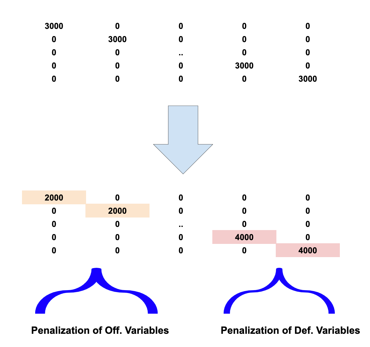
Doing it this way, we find that we get increased predictive accuracy when lowering the offensive penalization value, indicating that players have more influence on the offensive outcome of a possession.

This means that we allow for a wider spectrum of offensive impact values.

---

More tricks: Bayesian priors

So far, we’ve relied exclusively on matchup data. Standard ridge regression pushes everyone’s rating towards zero.

But what if we could assign each player a different starting point — a prior — derived from information outside the lineup data?

If we can build a metric on a scale similar to RAPM using individual stats, the resulting RAPM ratings are likely to stabilize more quickly. This type of metric is generally called Statistical Plus-Minus (SPM).

A simple example: a seven-footer with high block rates, low assists, low 3-point attempt rates, and poor free-throw shooting — think Rudy Gobert — is more likely to be a defensive positive and offensive negative than someone with Steve Nash’s statistical profile.

Even with limited sample sizes, individual stats can help shift our prior assumptions in the right direction.

If multicollinearity is high for a pair like Gobert and Nash, the two would end up with almost the same rating using standard RAPM. By introducing Bayesian priors — distinct starting values for each player’s offensive and defensive ratings — we can better disentangle their impacts.

We can plug in Basketball-Reference’s BPM as a prior, though any box-score-based metric can work, provided it is on — or transformed to — the same scale. The prior in my own xRAPM incorporates not only box-score data, but also play-by-play and advanced defensive statistics.

To integrate these priors into our RAPM framework, we need to fill a vector with size: number of players * 2

with the first value in the vector corresponding to the first variable, and so on.

The final regression formula then becomes

In Python code, it that equates to

p1 = np.linalg.inv((np.dot(X_t, X) + alpha * I))
p2 = X_t.dot(y) + beta0.dot(alpha * I)
beta = p2.dot(p1)

---

Standard errors

Justin Jacobs has demonstrated a method for computing standard errors for RAPM. We can calculate these without lots of additional computation:

[rows, columns] = np.shape(X)
resids = y - X.dot(beta)
squard_error_sum = np.sum(resids**2)
variance = squared_error_sum * p1 / (rows - columns - 1)

---

Most likely solution

Because of the large number of variables, we have many degrees of freedom. The output we’re getting from our RAPM calculation is just one of millions of potential solutions. It represents the most likely solution, given the data.

Those who are curious, and have sufficient computing power, can plug the same data into probabilistic programming tools such as Stan or PyMC, which can give further insight into the world of probabilities of each rating.

---

Try it out yourself

A link to lineup data, in SQL format, and a fully functioning RAPM Python script can be found here.

---

The story continues … in the next article

With more and more individual data being made available by the NBA, All-in-One metrics that incorporate that data keep gaining ground in accuracy.

Given that the issue of noise and multicollinearity in lineup data will never truly go away, improving SPMs — and thus the priors we plug into APM — appears to be the primary way we will progress toward even more accurate player metrics.

So, the next article in this series will cover how to build your own stats-based SPM metric.

1. Any individual player data can serve as input here.

2. A made shot that didn’t involve a shooting foul. Or the last of a series of free throws.