
How to build an NBA draft model
We have choices to make

Statistical draft models have several big advantages, compared to scouts: They are not swayed by aesthetics or random events, such as game-winning shots in the NCAA tournament. And they can “analyze” all of NBA draft prospects quickly.
Like other advanced metrics, NBA draft models use machine learning methods to predict outcomes based on historical data. Most draft models help assign accurate weights to certain player actions. For example, a scout might know that an offensive rebound is more important than a defensive rebound, but how much more?
Draft models can easily internalize information on past prospects: Given that the entire point of the model is to make predictions about future prospects — while using past prospect data as a guide — a statistical model easily “remembers” which blend of player stats were a good predictor of success.
These models can also more easily adjust for age and strength of schedule, as we’ve shown here:
How to adjust college stats — featuring Caleb Wilson vs. Cameron Boozer

You already know college stats play a vital role when it comes to the NBA draft — a prospect’s numbers indicate his strengths, weaknesses, and future NBA production.
It’s no surprise then, that draft models can sometimes predict future stars — or busts — better than scouts and GMs.
But draft models aren’t perfect — human evaluators still retain advantages when it comes to evaluating fluidity, body language, injury proneness and other factors.
While it’s hard to estimate how much each NBA team is influenced by draft model input, recent selections indicate that some teams value it highly. For example, Reed Sheppard — a 6’3” guard who didn’t score much in the NCAA — probably doesn’t go No. 3 in 2024 without draft model input.
Today we’ll show what such a statistical NBA draft model looks like, where the pitfalls lie, and what model-design decisions can be made. We’ll also supply some of the data, so that potential readers can try things out for themselves.
What is a draft model trying to predict?
Key decision: Choosing a target variable
When building NBA player metrics, such as xRAPM or BPM, most, if not all, modern metrics have settled on trying to predict the same thing: a player’s influence on the team’s point differential when the player is on the court.
Doing it this way has several benefits:
We already imply, in the design, that we’re looking for difference-makers, not those who simply accumulate counting stats.
The scale of the results is intuitive to understand: A player with, say, a +4 rating would help outscore the opponent by 4 points — over an average player — if he were to play 100 possessions.
With draft models, this decision becomes a little more muddy. As a draft model creator, you’re faced with several design decisions. Choosing a sensible target variable is the first one:
Option 1: Predicting per-possession NBA impact
In this category, there are several metrics to choose from, including xRAPM and BPM.
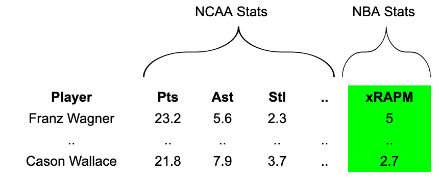
My personal preference here is to use a metric that has a box-score and a plus-minus component, such as xRAPM. The box-score component increases stability and makes the metric less susceptible to noise. The plus-minus component allows us to identify under-the-radar difference-makers such as Franz Wagner or Derrick White.
Our NCAA dataset contains every season since 2009-10. We’ll thus want to compute a 2011-2026 NBA metric to serve as our “ground truth.”
Our custom NBA metric has the usual suspects at the top: Jokić, LeBron, Curry, and so on. But these players aren’t relevant to the model, as they didn’t play in the NCAA after 2009-10, if at all.
Among the best players relevant to the model are Joel Embiid, Shai Gilgeous-Alexander, Dereck Lively II, and Dylan Harper. Some of the worst-rated players are Nick Smith Jr. and Jordan Hawkins.
Our data setup would look something like this:1
Among other downsides, one issue with predicting an impact metric is that some highly touted NCAA players who failed — such as Jahlil Okafor, James Wiseman and Anthony Bennett, who all rated -4 or worse — rip quite a big hole into our projections. With the average outcome being relatively far in the red, the projections for new prospects remain fairly low.
The fact that some of these former high draft picks were this bad is also not really relevant to us: Any player below somewhere around -1 should not find himself in the regular rotation of a winning team. So, whether he’s ultimately rated as -1 or -4 is moot: From the perspective of a drafting team, neither player should be in its long-term plans, and drafting such a player would count as a failure.
Option 2: Predicting “Wins”
The above metrics don’t take into account playing time — durability is not considered since the metrics try to predict per-possession impact.
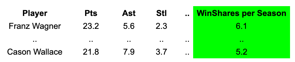
If we wanted to account for playing time, we could use metrics such as Win Shares or VORP, derived from Box Plus-Minus (both can be found at Basketball Reference).
Both of these estimate how many wins a player has added to the team’s season total:
When I worked for the Phoenix Suns and Dallas Mavericks, my colleagues in the analytics department sometimes opted for this approach, but I think there is a significant drawback: Players on bad teams can get too much credit.
The issue is that some teams give their young players more playing time — look at the Washington Wizards, for instance. In turn, that leads to those players getting more credit, not because they are better or more durable, but just because of the opportunities they were granted. In some cases, the issue is the team is below average at drafting and/or developing players.
Should the model really boost players picked by losing teams like, say, the Wizards or the Sacramento Kings? It seems like we’d be introducing a bias, and in the wrong direction.
Option 3: Predicting probabilities
Alternatively, we can try to predict a probability — for example, predicting whether a player will rate as above “0” in the impact metrics, such as xRAPM.
Cutoffs can be chosen at will, leading to different models and coefficients.
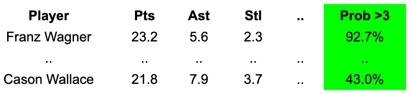
For the purposes of this article, I decided to predict four potential outcomes for each prospect:
Player impact below 0: This group is made up of players who shouldn’t be in a winning team’s long-term plans.
0 to 1.5: Typically a starter on a good team or maybe the best player on a bad team.
1.5 to 3: Often one of the three best players on a contender, peaking as a top-20 NBA player.
Above 3: High-impact players, including superstars.
I like this approach for a couple of reasons:
It better encapsulates the variance of outcomes. Player A might be more likely than Player B to be above average, but B might be more likely to become a star.
It solves the problem of extremely low-impact players in Option 1.
Does this approach imply that our target variable is just 1s and 0s — indicating whether a player’s impact has been above certain threshold, or below?
Machine learning algorithms tend not to love that particular data setup. It’s also not quite correct once we consider confidence in our estimates as measured by standard errors.
Take, for example, Cason Wallace, rated by the NBA impact model at +2.7. If we’re building a draft model that tries to predict if a player will surpass +3, then the target variable corresponding to Wallace would be a flat “0” when not considering standard errors.
But the +2.7 represents only our “best guess.” The level of uncertainty in that estimate is expressed by the standard error — in Wallace’s case the SE is 1.5 — creating a situation best displayed in the following graph:
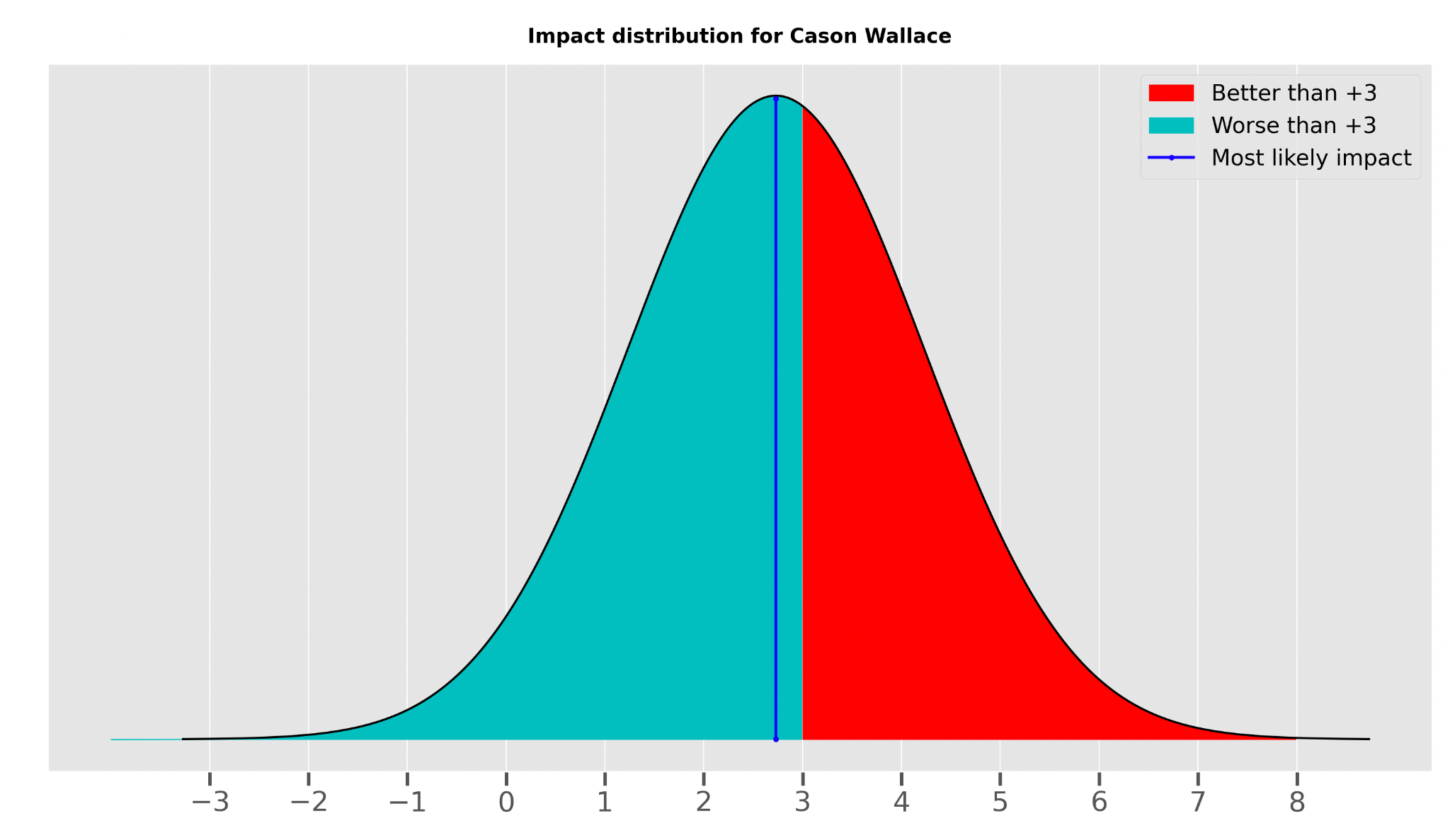
Incorporating these standard errors, we attain a value for a probability that Wallace is above +3: around 43%.2
One further consideration with this model and Option 1 is what to do with players who have seen very limited time in the NBA.
Per-possession metrics might not be harsh enough on certain players such as Usman Garuba, a 2021 first-round pick of the Houston Rockets, who rates as a ±0 in our custom impact metric.
Should a player who totaled just 1,228 minutes in three NBA seasons really serve as a positive example? While the answer is probably “no,” the solution isn’t so straightforward and requires some arbitrary cutoffs. Do we consider a player with less than 500 minutes per season a failed draft pick? 700?
What variables do we want to use?
Draft models try to make predictions based on historical data. But there are, of course, different types of data.
Do we include NCAA per-game data? Per possession? Totals?
My personal preference is to use estimates for each player’s “true skill.”
There are also intrinsic variables we can add. Among those are:
age
height
whether the player was born outside the U.S.
whether the player’s dad (or another family member) has played in the NBA
And we can add variables such as the quality of the team and its strength of schedule.
Note that some of these statistics have to be normalized — for example, “z-scored” — while others should exist as simple dummy variables.
Another big topic of debate is to whether to include past “pick number” information in the model.
One reason to do that: For players like Anthony Edwards — who had so-so college stats — scouts can identify attributes that a draft model isn’t able to see. For the current draft class, the player’s current draft board (or mock draft) rank would serve as a proxy.
Incorporating past draft pick information would make this a bit less of a “statistical” draft model, since we would be essentially including past scout/GM rankings, and we will rely on similar draft board information to make predictions.
On the plus side, this makes the model more accurate when predicting future success, since not everything is captured by the stats, and scout/GM evaluations add valuable information.
Not including draft pick information means the model stays “pure,” but the predictions will be a bit less accurate.
Which route you want to choose depends on your goals. Here’s a (paraphrased) discussion between me and the Suns’ director of analytics in 2013:
Me: “We can present the model with draft pick information included, which will make it more accurate. And the model results will align more with public opinion, giving us more credibility.”
Him: “Given that the influence of our analytics department is already small, we don’t want to mix our opinion with the scouts’ takes, since it would reduce our influence even further.”
Results
Which variables are most important?
Given that we are running three different models — for each group of players, based on their probability of becoming a star, a bust, and so on — we are getting three different set of coefficients.
Here are the most important ones:
Being an international prospect is a huge plus in regards to having an NBA impact rating above zero, but its importance diminishes with higher cutoffs.
Free-throw percentage and 2-point percentage are the most important shooting-related factors, and they remain relatively stable in importance.
Assists and height remain important with any cutoff.
Steals and blocks go in opposite directions:
Steals are important for becoming a >0 player, but they lose importance with higher cutoffs.
Blocks, on the other hand, gain importance with higher cutoffs.
Lastly, draft pick number is extremely important and gains in relative importance with higher cutoffs, indicating that the draft model has an easier time identifying solid players than superstars.
Here are, according to the model, the strongest NCAA seasons since 2010.
These represent “in-sample” results: We are asking what the model’s output would be, using hindsight, if presented with the following players today.
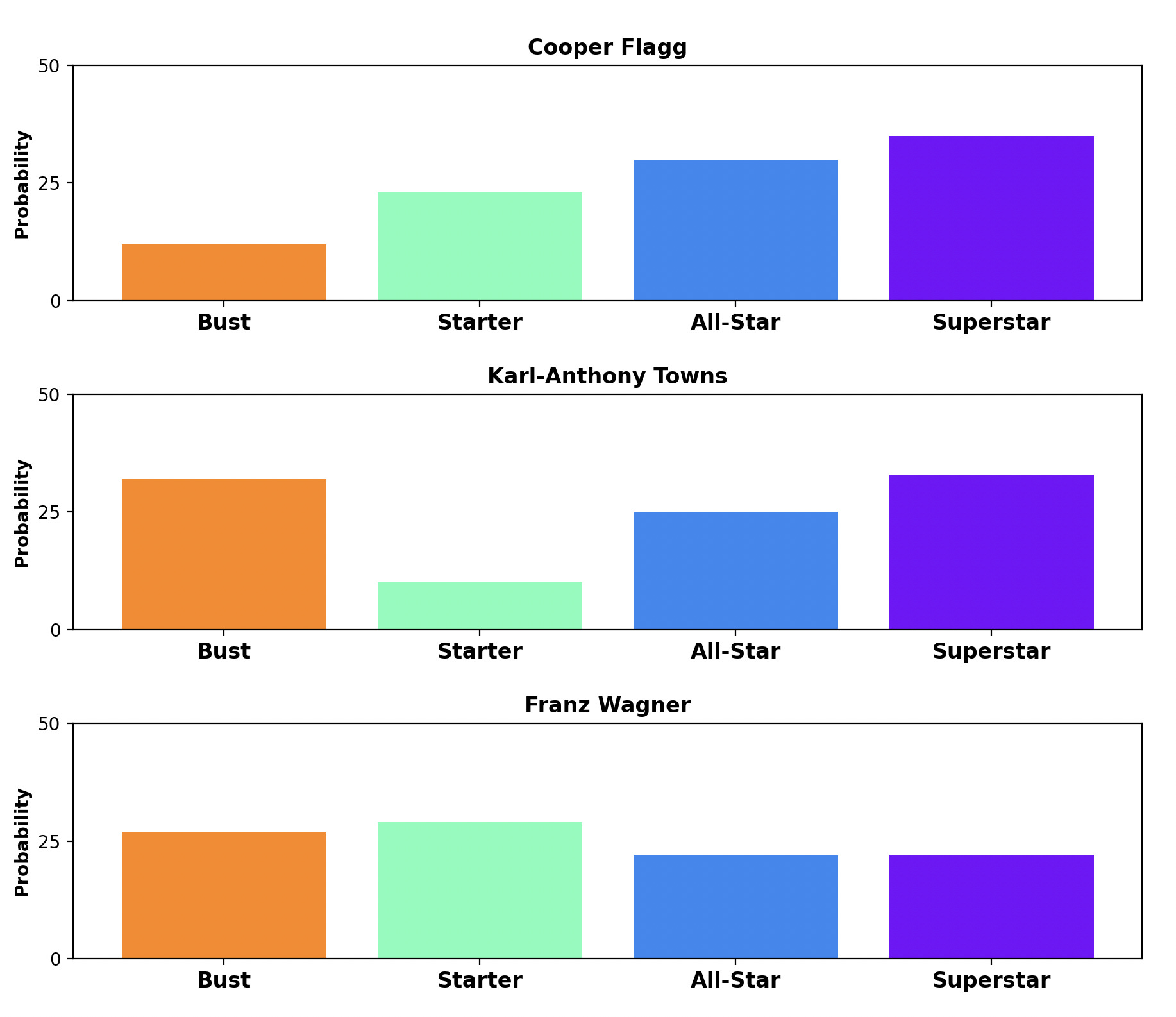
The following chart shows how the group predictions can vary wildly from player to player. In this example, Karl-Anthony Towns and Cooper Flagg were “predicted” to have a similar chance of becoming a superstar. But KAT had a significantly higher chance of becoming a bust.
Meanwhile, Franz Wagner had a lower “bust probability” than Towns, but the model saw less upside for Wagner and suggested he would most likely end up in the “Starter” group.
While we will present results for the 2026 draft class in a separate article, here is a Google doc containing past and current data that you can use to build a draft model on your own, and make projections for the 2026 draft class.
Player stats are per 100 possessions.
Using the inverse normal distribution.
 | A guest post by
|
According to my first ever built model. Aday Mara will be the steal of the first round and Cameron Boozer is the best player in this draft. Thanks for this can’t wait to keep playing with it.
The Model uses a Gradient Boosting Regressor trained on 719 NCAA prospects (2010–2025) with 18 features including per-100-possession shooting splits, playmaking, age, height, strength of schedule, and recruit rank percentile. It predicts per-possession NBA impact, then converts that to probabilities across 4 outcome tiers.
Cameron Boozer — +2.15 impact, 23.8% superstar probability
Aday Mara — +1.07, projects as likely starter/all-star ceiling
Allen Graves & Caleb Wilson — solid starter projections
How are you thinking about the timeline of the target variable? At first pass, I figure it makes sense to try to predict career peaks or totals of whatever the target is, but from a drafting team’s perspective, the decision-relevant window is probably relatively narrower, right?
Would you consider limiting the target to 3rd or 4th season impact (or something) to reflect the rookie extension decision point that teams have to make? Any drawbacks you’ve come across here?