
How to build an NBA box-score metric

Modern NBA metrics consist of two parts:
One that uses lineup data (aka plus-minus), which is how a team performs with a player or set of players on the floor.
Another that uses individual player stats, including those found in the box score.
Lineup data can, in theory, account for every action that make a difference on a basketball court. But it can be extremely noisy and requires a larger sample size.
Individual stats — points, rebounds, assists, etc. — are less susceptible to noise and stabilize a lot faster.
If we want to estimate a player’s impact as accurately as possible —- even if (and especially when) the sample size is limited —- we need to make use of all the available data.
Creating a box-score metric, similar to Basketball Reference’s BPM, is a crucial step in the process.
This article will show you how.
What we’re trying to find
With advanced metrics, we want to come up with a rating for each player on both ends of the floor.
Metrics using individual data — we’ll call them box-score metrics for now — do one thing at their core: They multiply individual player stats with weights and then add them up, leading to two numbers per player, denoting the player’s impact on offense and defense.1
Our job is to find a set of weights so that the player’s resulting rating predicts his on-court impact.
To avoid using subjective estimates — which would prove suboptimal in generating accurate metrics — we need techniques for generating these weights objectively.
We can thank Dan Rosenbaum for coming up with the following method:
Each player serves as one observation in our dataset.
The variables are the different individual stats.
The target variable is the player’s impact as measured by a metric that doesn’t contain any individual data.
Rosenbaum dubbed this approach “statistical plus/minus” in 2004.
The approach we present today follows in Dan’s footsteps, but with more modern techniques.
Which individual stats do we put in the model?
While the NBA box score provides the starting point, we can incorporate other stats as well.
Thanks to the NBA, we have new stats being recorded and published these days — deflections, screen assists, box-outs and many more. Some of these are derived from optical tracking, which didn’t exist when Rosenbaum originated SPM.
Beyond that, we can extract stats from NBA play-by-play data. For instance, I include kicked balls and goaltends, and I split blocked shots into two categories, depending on whether the offense or defense got the rebound.
For those who have access to raw camera data — as I did at the Dallas Mavericks — the possibilities seem almost endless: One could potentially extract how often a player misses a closeout or trails behind on an opponent fast break.
An important note: As we’ll see later, it makes sense to emphasize extracting defensive statistics more than offensive stats.
As stats come in different flavors — totals, per game, per 36 minutes, per 100 possessions, rate stats, etc. — one will have to make a decision on what to use here. My personal preference is to use the stats generated with this technique:
What’s the target variable?
As a target variable, we need a metric that a) captures the player’s impact, but also b) doesn’t include any box-score info while doing so.
That’s why we use pure lineup metrics for this step.
Lineup metrics also come in many different variations, including raw plus-minus, on-off, APM and RAPM.
Of the above, RAPM performs best at predicting out-of-sample data, so that’ll be our go-to target variable. The scale of the resulting metric will consequently mirror RAPM: Impact is measured in “influence on team points per 100 possessions,” with values around 3 and above denoting the player is a superstar.
In a way, we are treating RAPM as the ground truth. As you’ll see later, we will try to account for some of its deficiencies.
One interesting side product of this approach is that — for players where we have both an SPM and an RAPM rating — we can determine which players are high in fiber or high in fluff. More on that below.
The general practice has been to use multi-season RAPM when generating the weights, as that increases predictive accuracy. As most of NBA.com’s advanced stats go back to 2016-17, we will be using RAPM from 2016-17 to 2025-26 for this exercise.
Since we are now using 10 years of RAPM, the individual data needs to match that same time frame: For each player in the sample, we will want to compute their 10-year “averages” across the same decade.
And because 10 years is rather long, I am using an age adjustment in RAPM, which boosts the ratings of players who play with really old or young teammates.
Take, for example, LeBron James and the Lakers. Because he is seen as a single entity across the 10-year dataset, we have to adjust his current teammates’ ratings to account for the fact that he’s 41 and not as good as he was for most of the past decade — the system gives his teammates a boost to avoid penalizing them for his decline.
As I showed in a previous article, an offensive player’s influence on the outcome of a possession is greater than that of a defender. Thus, using different penalization values for offense and defense makes sense.
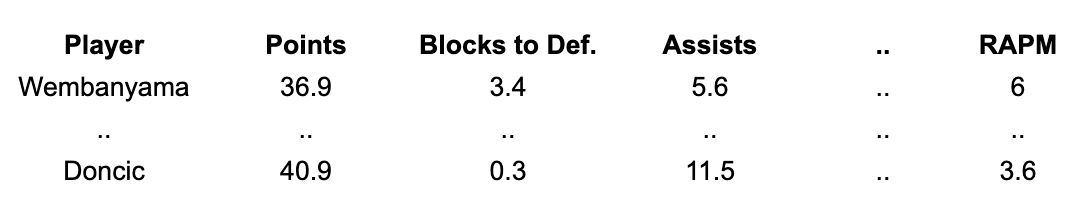
Here’s what our setup would look like if we used 2016-17 to 2025-26 per-possession stats and total RAPM:
Weighting individual observations
No matter what time frame you select, your population of players will have a wide range of minutes played — from a lot to a few.
Obviously, Nikola Jokić should have more influence when generating the weights compared to, say, Anthony Bennett: Jokić’s RAPM is more accurate (with lower standard error), and we also have a more accurate grasp of his “true” career skill for each stat.
Simply from a machine learning standpoint, we want to rely more strongly on more accurate observations.
In the past, this situation was often dealt with by choosing a minutes cutoff, removing those players below the cutoff from the sample, and weighting the remaining observations equally.
But it’s rather arbitrary to give a player with, say, 1,001 minutes the same weight as another player with 20,000 minutes, while another player with 999 minutes might not have any influence whatsoever.
Fortunately, there is a better way: Keep all of the observations in the sample and weight them according to their RAPM standard error — that is, the level of uncertainty we have in their RAPM estimate.
As with box-score statistics, RAPM estimates come with their own measure of uncertainty. We get the standard errors through a technique developed by Justin Jacobs.
For the players in our RAPM sample, the standard errors look like this:
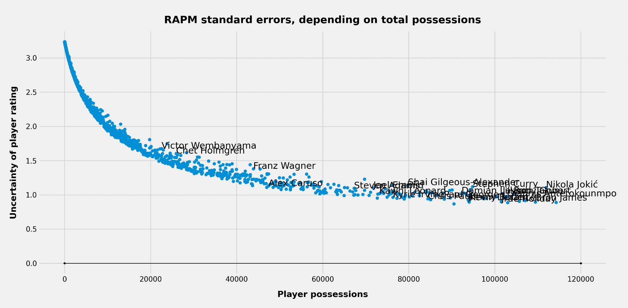
As expected, the uncertainty goes down with more possessions played. But it isn’t a linear relationship: We first get a steep decline with the initial possessions, but the curve tends to flatten out with more possessions.
The player with the lowest standard error should be given the largest weight. In our case that is Dennis Schröder. He has not played the most minutes in the sample, but because he’s a journeyman whose career includes the entire 10-year span, he’s played with hundreds of teammates, making us more confident in his RAPM estimate.
A player with close to zero minutes should be given a weight extremely close to 0. Later, the weights will have to be normalized so that the average weight is 1. Schröder ends up with a relative weight of around 3.
What’s omitted
Box Plus-Minus (BPM) is the best-known public version of SPM, as it’s published at Basketball Reference.
In contrast to BPM, several aspects have been kept simple in our version of SPM:
There is no positional or role adjustment.
There are no team adjustments.
No team-related stats are required.
Stat normalization
There is one final pre-processing step: normalization of the different stats.
Instead of inputting, say, per-100 estimates into the regression, we are instead transforming each column to have an average of 0 and a standard deviation of 1.
For example, let’s take Victor Wembanyama: His block rate2 is eight standard deviations above the average posted by an average NBA player.
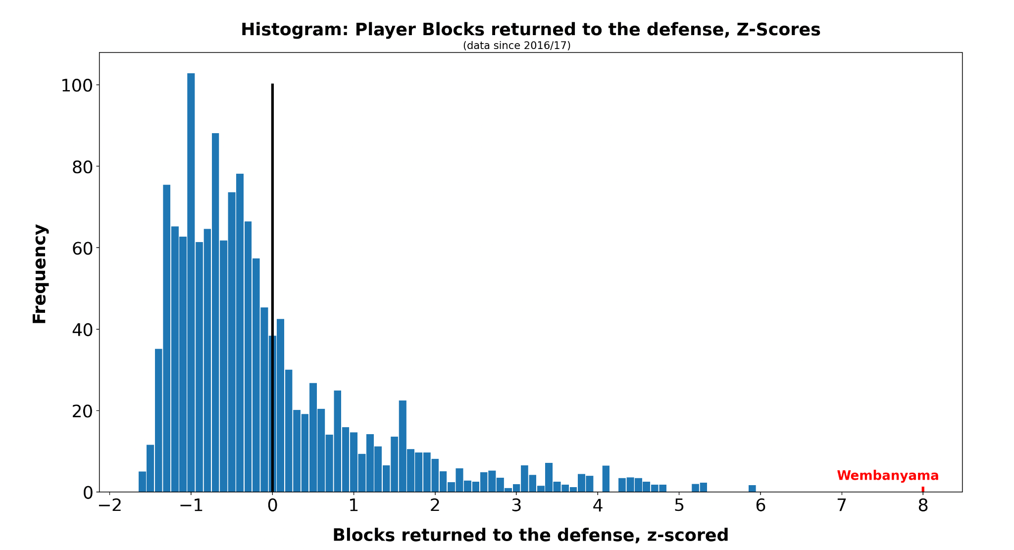
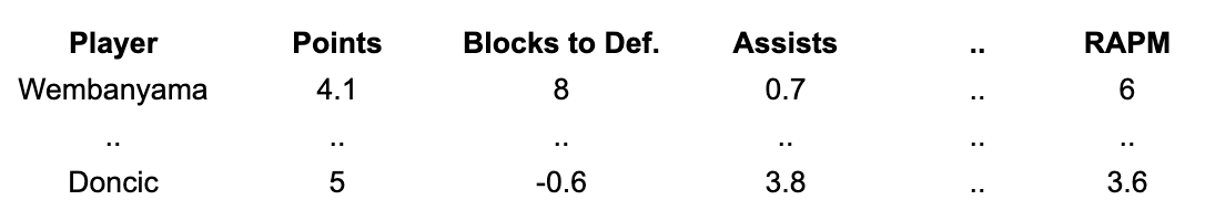
This technique is called “z-scoring” and generally helps machine learning algorithms to perform better. The resulting setup then looks a little different:
Results
While this data setup can — like others we’ve previously presented — be put into many different machine learning algorithms, using regression has the benefit of telling us the relative importance of the different stats.
We get two immediate results from running the regression:
A weight for each stat — this can be positive or negative.
An SPM rating for each player (for the 10-year period we chose).
Because we run the analysis for both offense and defense separately, we get two sets of weights.
The analysis says that being above average at the following stats leads to higher offensive impact: minutes played; and points, offensive rebounds and assists per 100 possessions.
Low turnover numbers — especially dead-ball turnovers — and low block numbers are also positive indicators.
That last one might be surprising, but it’s an example of how advanced metrics can find and employ indirect signals.
Players with fewer offensive skills often take a different path to the NBA — through their defensive impact. That’s especially true for bigs.
The regression picks up this selection bias: Players with high block numbers might otherwise not even be in the NBA — if not for their rim protection — as they tend to lack passing and shooting skills.
On the defensive end, forcing misses near the basket, defensive-rebounding 2-pointers, blocking shots that go to the defense and drawing charges are the biggest positive indicators.
Defensive rebounds off of free throws are a negative indicator, probably because they signify a tendency to “stat-stuff.” And three categories that make opponent fast breaks more likely are also negatives on defense — blocked shots against, live-ball turnovers and offensive rebounds.
Using these weights, we can easily compute 10-year SPM ratings:
Another consideration is which machine learning algorithm to choose when running the analysis.
Disclaimer: We should not be using whichever machine learning method maximizes in-sample correlation. Instead, we want to find the ML method that minimizes leave-one-out prediction error: Training the model on all samples but 1, then predicting this player’s RAPM, how far off are we from his actual RAPM?
That said, in-sample comparison of SPM vs. RAPM gives us a good visual representation that defensive SPM metrics tend to struggle more when estimating impact.
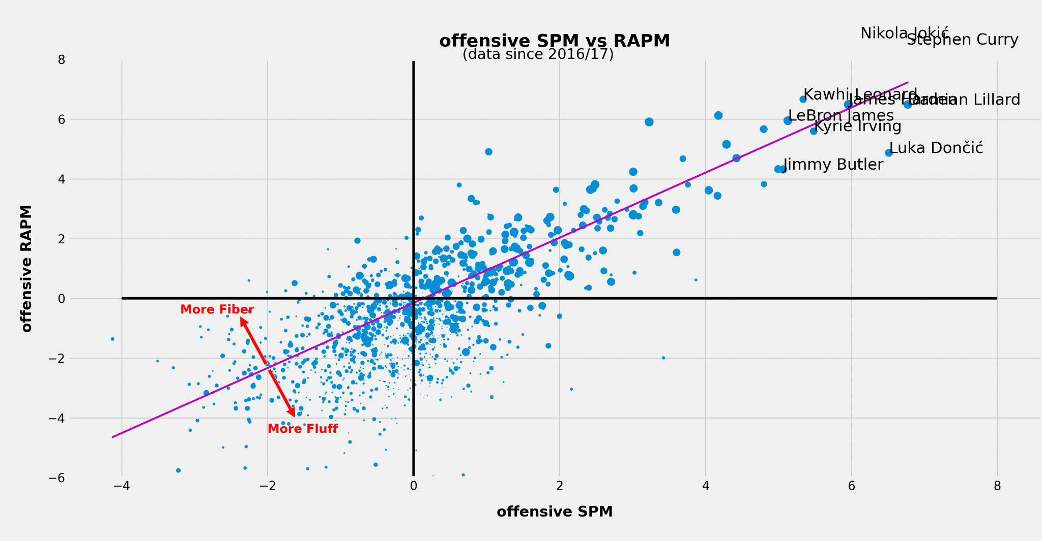
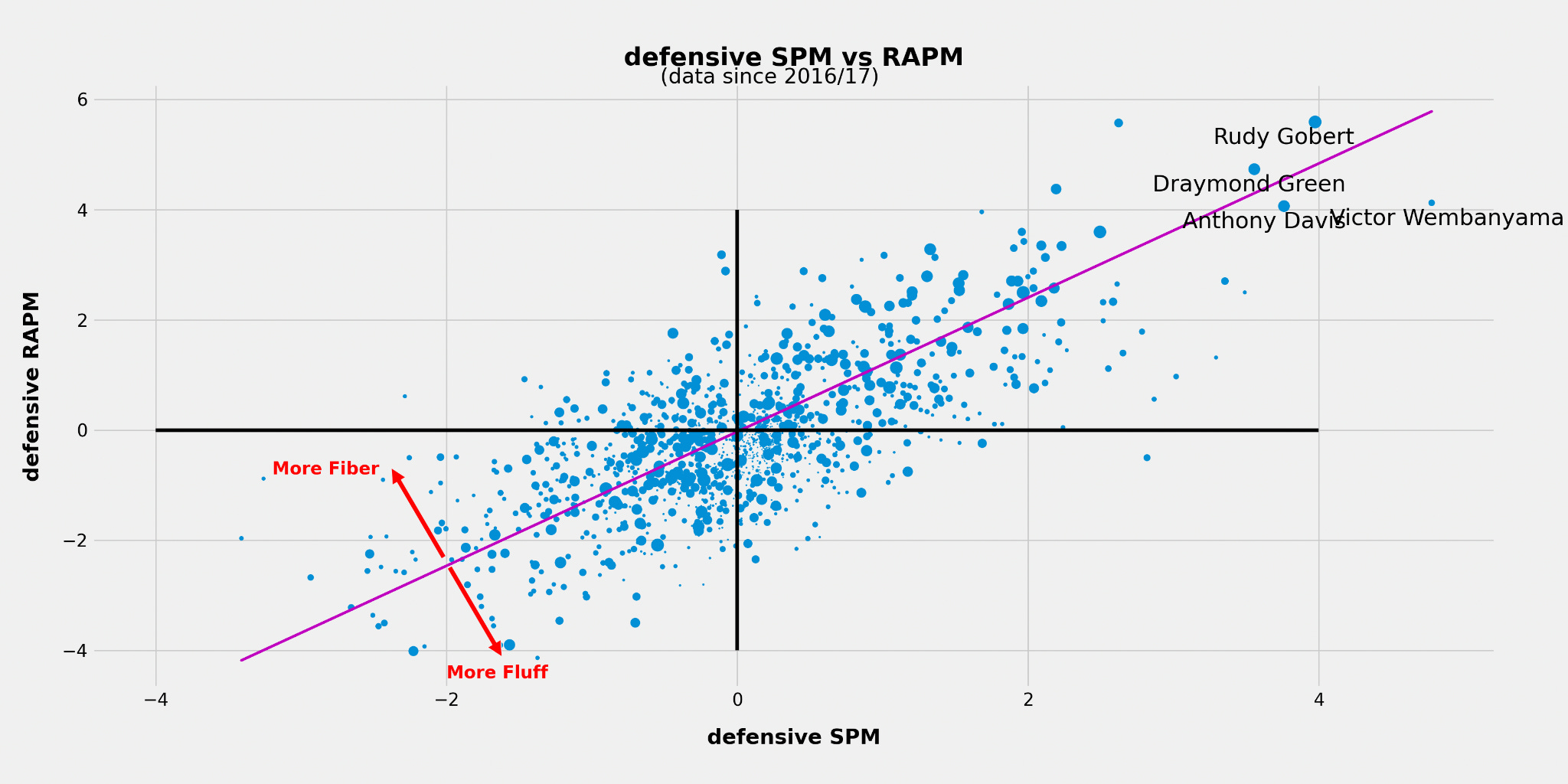
The most likely reason is that the individual stats we have are less capable of capturing actual defensive impact relative to how well offensive stats capture offensive impact.
This is especially true without NBA advanced and play-by-play data: The only defensive stats in the box score are rebounds, blocks and steals.
Fluff vs. Fiber
These charts also help us identify high-fluff and high-fiber players:
Those far below the line tend to have a significantly higher SPM rating than RAPM. When the difference is extreme, that indicates the player might be doing things that can be counted but doesn’t “do the little things” that lead to winning.
Players above the line, on the other hand, tend to get underrated by SPM — their plus-minus often outpaces their countable contributions.
Single-season SPM
Using the weights, we can also compute SPM ratings for shorter time periods — single seasons, for example.
For the 2025-26 regular season, pure SPM ratings have these players at the top:
How to combine SPM with RAPM
Combining both methods gives us the best of both worlds: SPM is less susceptible to noise, and ideally RAPM captures what SPM has missed.
If we want to create a metric that’s optimized for predicting the immediate future, here is the approach that I found to be most accurate:
Employing the SPM impact estimates as Bayesian priors, we use about 2-3 years of lineup data to compute “prior-informed RAPM.”3
How much deviation we allow from these priors is ultimately an empirical question: If our SPM was perfect, and our lineup data was very noisy, we’d allow zero deviation (infinite penalization). With less accurate SPM and more accurate lineup data, the penalization gets reduced.
DIY
For those readers who want to run the analysis for themselves, we’ve compiled the data in a Google spreadsheet.
This includes 10 years of box-score, play-by-play and advanced data from NBA.com.4
Also included are the RAPM estimates and the corresponding standard errors.
Below, we will also refer to box-score metrics as SPM.
Blocks rebounded by the defense, that is.
Standard RAPM inherently uses 0 as a prior for each player’s rating.
Most of the data is supplied as totals over the 10-year time frame. There might be slight discrepancies with official data, as some stats are extracted from play-by-play data, which isn’t available for every game.
 | A guest post by
|
Hi, really interested in this! How do I find the other articles part of this series?