


Two weeks into the NBA season, we’re starting to see real results.
The very best tools we have for analyzing winning and losing in the NBA are advanced stats, and my contributions to the field include xRAPM and the related family of impact metrics.
Now that xRAPM is up and running for 2026-27, today let’s look at the metric itself: where it comes from, how it works, why it’s helpful, and how to use it.
And for the really juicy stuff, in an upcoming article I’ll examine what the early results mean for some of the NBA’s greatest stars — for better and worse.
The two major elements of NBA impact metrics
xRAPM and other leading impact metrics typically consist of two major elements: box-score stats and lineup stats.
Most of these metrics include splits for offense and defense.
Box-score-based metrics
Before the current crop of modern impact metrics was born, some enterprising analysts found ways to use basic stats to analyze basketball.
Analytics pioneers like Dean Oliver and John Hollinger created advanced metrics from the box score: They combined points, rebounds, assists, and so on with game pace to provide new tools for evaluating players and teams.
For example, True Shooting percentage is a relatively simple but effective way to assess shooting efficiency. It accounts for trips to the line and the extra value of a 3 over a 2.
More broadly, all-in-one metrics like PER and Win Shares, developed by Hollinger and Justin Kubatko (building on Oliver’s work), respectively, multiplied box-score (and derived advanced) stats with weights to arrive at a single number per player.1
In the same time frame, Dan Rosenbaum came up with the idea to use machine learning to determine the optimal set of weights, giving birth to Statistical Plus-Minus (SPM) — a forerunner to the similar Box Plus-Minus (BPM) devised by Daniel Myers and found at Basketball Reference.
Because the weights were now determined objectively, with the help of computers, and with the main goal of maximizing prediction accuracy, metrics got better at forecasting.

Another benefit of these SPM-type metrics is that weights could continually be updated. In a league with constant rule changes, this was necessary to ensure predictive accuracy.
Further developments in this direction came from integrating additional data. Since the advent of tracking cameras, more player stats have been made available to the public.
The drawbacks of these metrics tend to relate to statistical blind spots: Some of “the little things” players do — plays which influence winning and losing — still often aren’t covered by individual statistics. For instance, arguing with the referee while the rest of your team defends 4-on-5 is not captured by any particular counting stat.
Statistical tests made it evident early on that the traditional box score alone gave us a fairly accurate picture of a player’s offensive abilities and his impact. Defense, though, is another story.
The box score has only three true defensive categories. And each can be inflated by players, even to the point of being detrimental to team success. For example, players can gamble for steals, leaving gaps in the defense when the gamble doesn’t pay off. Same goes for blocked shots. Or they can chase defensive rebounds, forgoing their duty to box out.
Therefore, integrating individual defensive stats derived from optical tracking tends to give plenty of bang for the buck when improving modern NBA metrics.
This includes stats such as …
screen assists
deflections
box-outs
defender FG% (FG% when a certain defender is near the shooter)
loose balls recovered
charges drawn
These SPM-type metrics also have the benefit of objectively telling us which actions are most meaningful when it comes to impacting winning.
On the offensive side, these things are most closely connected to high impact:
scoring a lot, and efficiently
creating assists
offensive rebounding
spacing the floor
not turning the ball over (”dead-ball” turnovers are strongly connected with hurting team offense)
And on defense:
forcing opponent misses (forcing misses near the basket gives extra credit to the defender)
defensive rebounds off of 2-pointers (but not FTs or 3s)
blocks that go to the defense
getting deflections and charges
avoiding live-ball turnovers
avoiding missed 2-point FGs (missed 2s and live-ball turnovers appear more likely to lead to an opponent fast-break)
Plus-minus metrics
To have an objective measure which we can then use to find optimal weights (for SPM), we needed another metric that we could derive from data that included none of these box-score stats.
Enter the plus-minus family of statistics.
The simple version of plus-minus — found in the box score starting around 2007 — measures how many points a team outscored its opponents by while the player in question was on the court.
The immediate drawback here is that simply sharing court time with strong teammates can lead to a positive plus-minus.
The cousin of standard plus-minus, “on-off” measures how well the team did with you, compared to without you. Along similar lines, it is highly dependent on who you play with, and who subs in and out for you.
Adjusted plus-minus (APM), developed by Wayne Winston and Jeff Sagarin and, separately, Dan Rosenbaum, adjusts for the quality of a player’s teammates and opponents, using the lineups on the floor throughout each game. Later on, models also adjusted for the state of the game.2
For deeper dives on this topic, see these free articles:


The results of these APM-type metrics served a pair of purposes:
One, they created an objective measure to help generate weights in the aforementioned SPM.
Two, APM should be able to capture all of the actions that influence the outcome of a basketball game, even the smallest things.
But randomness also has a big influence on the outcome. A player can get lucky by being on the court during, for instance, a big run fueled by 3-pointers, and subsequently get a lot of unwarranted credit.
Lineup-based metrics can thus stay quite inaccurate for relatively long periods of time. This is one reason why — when generating a lineup metric to estimate weights for SPM — multi-year APM is used, in order to increase sample size and thus decrease statistical noise.3
A further breakthrough came in the form of using a more modern machine-learning approach — called ridge regression — which nudges player ratings towards zero and significantly increases accuracy.
This development came in 2010, when Joe Sill won a best paper prize at the Sloan Sports Analytics Conference. RAPM (Regularized Adjusted Plus-Minus) was born.
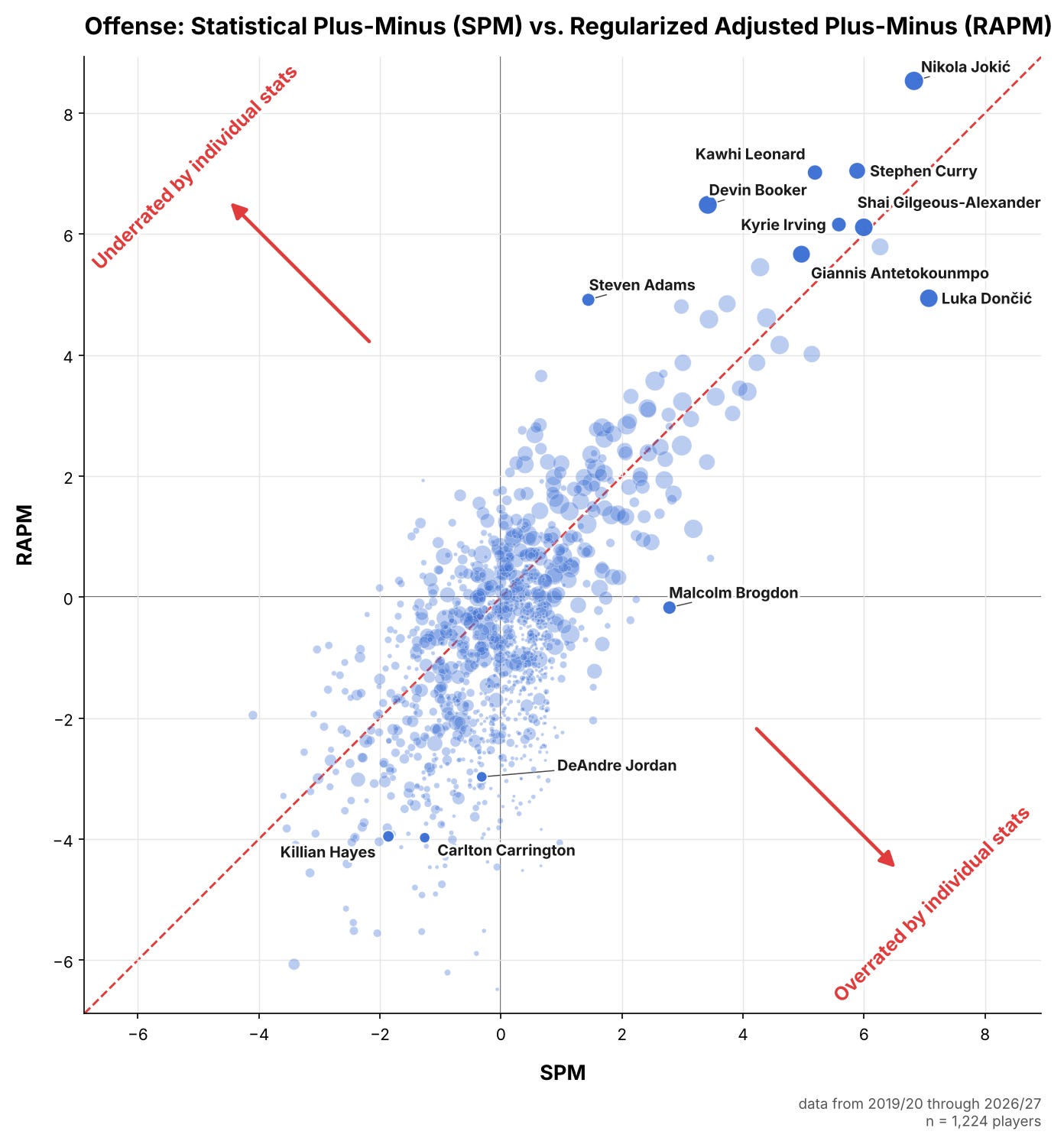
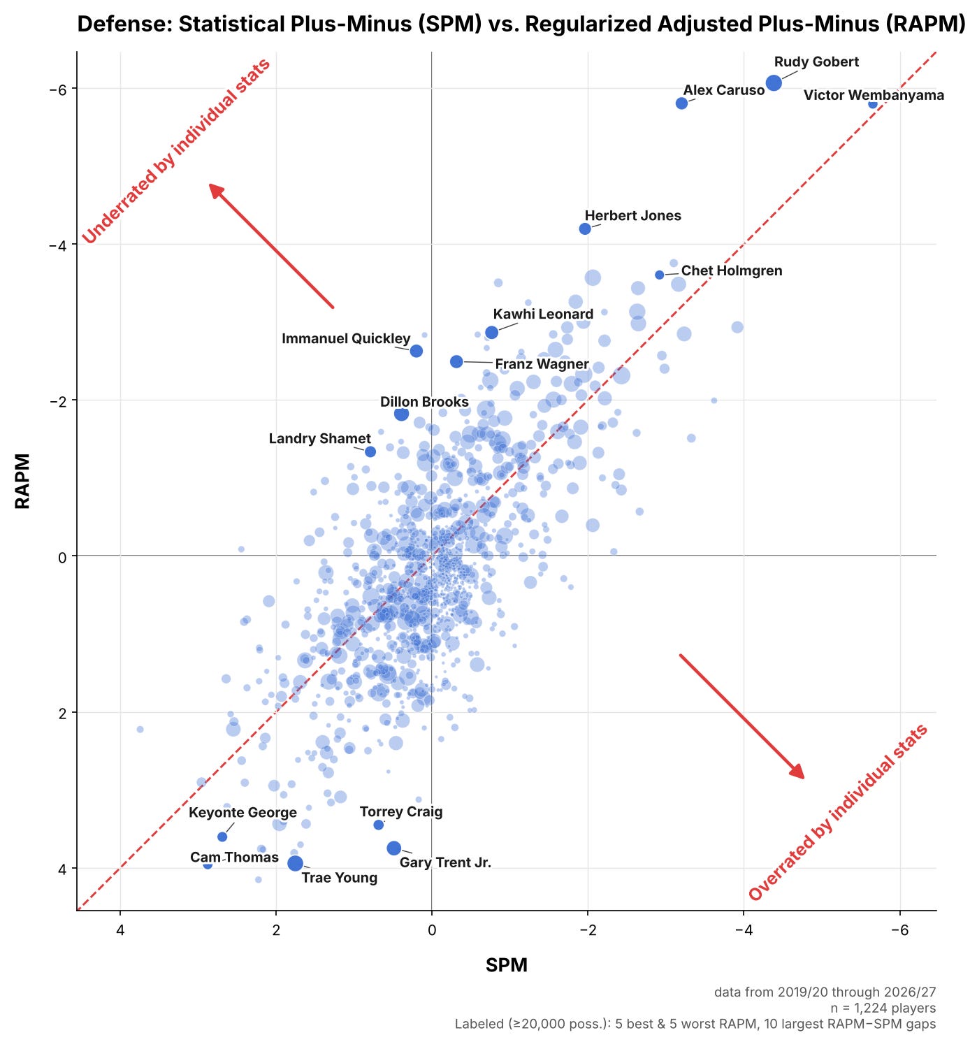
How players stack up in these two metric families, SPM and RAPM, can be seen in the following charts, which show the results for offense and defense.
Note that — for sample size and accuracy — the time period covered here runs from 2019-20 to 2026-27:
The best of both worlds
We now had two distinct parts: One set of metrics based on individual stats that struggled to capture the little things, and another that captured the little things and could not be misled by stat-stuffing — but which struggled with noise in the raw data.
But RAPM gives every player a starting point of zero, which they get pushed towards. That “0” can be replaced with a more accurate, individual starting point, which stems from SPM. Then, we add information from lineup data to nudge the numbers slightly in the direction that seems more correct. This is the design of my own xRAPM.
Take, for example, Alex Caruso: His teams have always defended better with him on the court. But measures derived from box scores don’t directly capture his ball denial and ability to cut off lanes. His defensive SPM, then, lags behind.
But because we have an overwhelming amount of lineup data pointing towards Caruso’s elite impact, he gets a boost in the final metric.
How to use xRAPM
xRAPM’s results for 2026-27 can be found at my site, xRAPM.com. These will be updated regularly.
While there are various versions — the pure lineup-based estimate is here, team rankings are here,4 and you can find much more at the site — the numbers on the main page have been proven to be the most accurate at predicting future outcomes.
Here’s how to read what you see there:
From the perspective of these metrics, offensive impact and defensive impact are additive. And each number is calculated to be “relative to a league-average player.” In other words, the average player rates as zero (0.0).
For example, Victor Wembanyama’s defensive xRAPM is currently estimated at -7.5, which means a lineup with Wemby alongside four average defenders would allow 7.5 fewer points per 100 possessions than an average lineup: 106 points, instead of 113.5.56
Our free series of technical articles:


The actual calculations are more complex — among other things, they adjust for team pace. Win Shares also builds on team offensive and defensive ratings.
This includes incorporating the “rubber band effect,” identified by Matthew Goldman and Justin M. Rao, in which teams that are ahead ease off and teams that are behind push harder, as I covered in more detail in this piece.
aka standard error
Adjusted for strength of schedule.
As of November 5.
Assuming neither team is significantly ahead or behind.
